Przejdź do głównej zawartości

Jak połączyć komórki, jeśli ta sama wartość istnieje w innej kolumnie w programie Excel?

Jak pokazano na poniższym zrzucie ekranu, jeśli chcesz połączyć komórki w drugiej kolumnie na podstawie tych samych wartości w pierwszej kolumnie, możesz użyć kilku metod. W tym artykule przedstawimy trzy sposoby wykonania tego zadania.

połącz, jeśli to samo


Połącz komórki, jeśli mają taką samą wartość, z formułami i filtrem

Poniższe formuły ułatwiają łączenie zawartości odpowiednich komórek w kolumnie na podstawie tej samej wartości w innej kolumnie.

1. Wybierz pustą komórkę obok drugiej kolumny (tutaj wybieramy komórkę C2), wprowadź formułę = JEŻELI (A2 <> A1, B2, C1 & "," i B2) do paska formuły, a następnie naciśnij klawisz Wchodzę klawisz.

2. Następnie wybierz komórkę C2 i przeciągnij Uchwyt Wypełnienia w dół do komórek, które chcesz połączyć.

3. Wprowadź wzór = JEŻELI (A2 <> A3, ZŁĄCZ.KATENATY (A2, "," "", C2, "" ""), "") do komórki D2 i przeciągnij uchwyt wypełnienia w dół do pozostałych komórek.

4. Wybierz komórkę D1 i kliknij Dane > FILTRY. Zobacz zrzut ekranu:

5. Kliknij strzałkę rozwijania w komórce D1, usuń zaznaczenie (Puste) a następnie kliknij OK przycisk.

Możesz zobaczyć, że komórki są połączone, jeśli wartości w pierwszej kolumnie są takie same.

Note: Aby z powodzeniem używać powyższych formuł, te same wartości w kolumnie A muszą być ciągłe.


Łatwo łącz komórki, jeśli ta sama wartość z Kutools for Excel (kilka kliknięć)

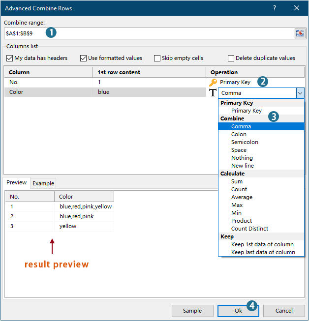
Metoda opisana powyżej wymaga utworzenia dwóch kolumn pomocniczych i obejmuje wiele kroków, co może być niewygodne. Jeśli szukasz prostszego sposobu, rozważ użycie metody Zaawansowane wiersze łączenia narzędzie od Kutools dla programu Excel. Za pomocą zaledwie kilku kliknięć to narzędzie umożliwia łączenie komórek przy użyciu określonego ogranicznika, dzięki czemu proces jest szybki i bezproblemowy.

Wskazówka: Przed zastosowaniem tego narzędzia zainstaluj Kutools dla programu Excel po pierwsze. Przejdź do bezpłatnego pobierania teraz.

1. kliknij Kutools > Połącz i podziel > Zaawansowane wiersze łączenia aby włączyć tę funkcję.
2. w Zaawansowane wiersze łączenia oknie dialogowym, wystarczy:
  • Wybierz zakres, który chcesz połączyć;
  • Ustaw kolumnę z takimi samymi wartościami jak Główny klucz Kolumna.
  • Określ separator, aby połączyć komórki.
  • Kliknij OK.

Wynik

Note:

Połącz komórki, jeśli mają taką samą wartość z kodem VBA

Możesz także użyć kodu VBA do łączenia komórek w kolumnie, jeśli ta sama wartość istnieje w innej kolumnie.

1. naciśnij inny + F11 klawisze, aby otworzyć Aplikacje Microsoft Visual Basic okno.

2. w Aplikacje Microsoft Visual Basic okno, kliknij wstawka > Moduł. Następnie skopiuj i wklej poniższy kod do pliku Moduł okno.

Kod VBA: łącz komórki, jeśli te same wartości

Sub ConcatenateCellsIfSameValues()
	Dim xCol As New Collection
	Dim xSrc As Variant
	Dim xRes() As Variant
	Dim I As Long
	Dim J As Long
	Dim xRg As Range
	xSrc    = Range("A1", Cells(Rows.Count, "A").End(xlUp)).Resize(, 2)
	Set xRg = Range("D1")
	On Error Resume Next
	For I = 2 To UBound(xSrc)
		xCol.Add xSrc(I, 1), TypeName(xSrc(I, 1)) & CStr(xSrc(I, 1))
	Next I
	On Error GoTo 0
	ReDim xRes(1 To xCol.Count + 1, 1 To 2)
	xRes(1, 1) = "No"
	xRes(1, 2) = "Combined Color"
	For I = 1 To xCol.Count
		xRes(I + 1, 1) = xCol(I)
		For J = 2 To UBound(xSrc)
			If xSrc(J, 1) = xRes(I + 1, 1) Then
				xRes(I + 1, 2) = xRes(I + 1, 2) & ", " & xSrc(J, 2)
			End If
		Next J
		xRes(I + 1, 2) = Mid(xRes(I + 1, 2), 2)
	Next I
	Set xRg = xRg.Resize(UBound(xRes, 1), UBound(xRes, 2))
	xRg.NumberFormat = "@"
	xRg = xRes
	xRg.EntireColumn.AutoFit
End Sub

Uwagi:

1. D1 W linii Ustaw xRg = Range („D1”) oznacza, że ​​wynik zostanie umieszczony począwszy od komórki D1.
2. "Nie" i „Połączony kolor” W linii xRes (1, 1) = "Nie" i xRes (1, 2) = "Połączony kolor" to nagłówki wybranych kolumn. 

3. wciśnij F5 klucz do uruchomienia kodu, otrzymasz połączone wyniki w określonym zakresie.


Łatwo łącz komórki, jeśli mają taką samą wartość z Kutools for Excel

Najlepsze narzędzia biurowe

🤖 Pomocnik AI Kutools: Zrewolucjonizuj analizę danych w oparciu o: Inteligentne wykonanie   |  Wygeneruj kod  |  Twórz niestandardowe formuły  |  Analizuj dane i generuj wykresy  |  Wywołaj funkcje Kutools...
Popularne funkcje: Znajdź, wyróżnij lub zidentyfikuj duplikaty   |  Usuń puste wiersze   |  Łącz kolumny lub komórki bez utraty danych   |   Okrągły bez wzoru ...
Super wyszukiwanie: Wiele kryteriów VLookup    Wiele wartości VLookup  |   Przeglądanie pionowe na wielu arkuszach   |   Wyszukiwanie rozmyte ....
Zaawansowana lista rozwijana: Szybko twórz listę rozwijaną   |  Zależna lista rozwijana   |  Lista rozwijana wielokrotnego wyboru ....
Menedżer kolumn: Dodaj określoną liczbę kolumn  |  Przesuń kolumny  |  Przełącz stan widoczności ukrytych kolumn  |  Porównaj zakresy i kolumny ...
Polecane funkcje: Fokus siatki   |  Widok projektu   |   Duży pasek formuły    Menedżer skoroszytów i arkuszy   |  Biblioteka zasobów (Automatyczny tekst)   |  Selektor dat   |  Połącz arkusze   |  Szyfruj/odszyfruj komórki    Wysyłaj e-maile według listy   |  Super filtr   |   Specjalny filtr (filtruj pogrubienie/kursywa/przekreślenie...) ...
15 najlepszych zestawów narzędzi12 Tekst Tools (Dodaj tekst, Usuń znaki, ...)   |   50 + Wykres rodzaje (Wykres Gantta, ...)   |   40+ Praktyczne Wzory (Oblicz wiek na podstawie urodzin, ...)   |   19 Wprowadzenie Tools (Wstaw kod QR, Wstaw obraz ze ścieżki, ...)   |   12 Konwersja Tools (Liczby na słowa, Przeliczanie walut, ...)   |   7 Połącz i podziel Tools (Zaawansowane wiersze łączenia, Podział komórki, ...)   |   ... i więcej

Zwiększ swoje umiejętności Excela dzięki Kutools for Excel i doświadcz wydajności jak nigdy dotąd. Kutools dla programu Excel oferuje ponad 300 zaawansowanych funkcji zwiększających produktywność i oszczędzających czas.  Kliknij tutaj, aby uzyskać funkcję, której najbardziej potrzebujesz...

Opis


Karta Office wprowadza interfejs z zakładkami do pakietu Office i znacznie ułatwia pracę

  • Włącz edycję i czytanie na kartach w programach Word, Excel, PowerPoint, Publisher, Access, Visio i Project.
  • Otwieraj i twórz wiele dokumentów w nowych kartach tego samego okna, a nie w nowych oknach.
  • Zwiększa produktywność o 50% i redukuje setki kliknięć myszką każdego dnia!
Comments (23)
No ratings yet. Be the first to rate!
This comment was minimized by the moderator on the site
thank you very much, the VBA code works very well but I have a question that I can't solve.

NO Color
1 red
1 blue
1 red
1 yellow
2 red
2 yellow


in this case, in column B we have some duplicate colors related to the same number. How can I have an output that only return the values once?

I would like an output like this

NO Color
1 red, blue, yellow
2 red, yellow
This comment was minimized by the moderator on the site
Hi

The second method described in the post can help you solve this problem. After following the steps to specify the settings, checking the Delect Duplicate Values option will delete all duplicates in the combined results.
https://www.extendoffice.com/images/stories/comments/comment-picture-zxm/concatenate.png
This comment was minimized by the moderator on the site
Thank you so much for this formula! It saved hours of investigation! Fantastic work :)
This comment was minimized by the moderator on the site
Hi Crystal,

Thanks for your reply. I'll have to put my thinking hat on again...
Thank you
This comment was minimized by the moderator on the site
Hello, the macro above works great! Thank you. Is it anyway possible (I tried, but not successful) to amend it to concatenate column B (description) based on duplicates in column A (HS code) but also taking column C (origin) in the combination?
So description texts concatenate per HS code per origin.
Also column D(quantity) and column E(value) must be summed per HS code and origin.

A B C D E
HS CODE DESCRIPTION ORIGIN QUANTITY VALUE
5407420000 TWEED CN 10 € 150,00
5407420000 COTTON CN 15 € 250,00
5407420000 POLYESTER TW 5 € 130,00
5407420000 ORGANIC COTTON US 18 € 450,00
5407420000 COTTON US 23 € 780,00
5407420000 VELVET DELUXE CN 20 € 380,00
5407420000 COTTON CN 10 € 120,00
5806310000 TWEED JP 15 € 35,00
5806310000 POLYESTER AU 20 € 78,00
5806310000 TWEED AU 25 € 254,00
5806310000 POLYESTER SG 130 € 888,00
5806310000 COTTON EU 120 € 945,00
5806310000 COTTON FABRIC EU 10 € 80,00


Result shopuld be:

5407420000 TWEED, COTTON, VELVET DULUXE, COTTON, CN 55 € 900,00
5407420000 POLYESTER TW 5 € 130,00
5407420000 ORGANIC COTTON, COTTON US 41 € 1230,00
5806310000 TWEED JP 15 € 35,00
5806310000 POLYESTER, TWEED AU 45 € 332,00
5806310000 POLYESTER SG 130 € 888,00
5806310000 COTTON, COTTON FABRIC EU 130 € 1025,00

I hope this possible, thank you!
This comment was minimized by the moderator on the site
Hi Ivar,

Thank you for your comment. I am not able to solve this problem with VBA code yet. Sorry for that.
You can try if the last method can help.
This comment was minimized by the moderator on the site
Hello, how would the VBA code be adjusted if I want to combine cells in column M based on the duplicates in column A?
This comment was minimized by the moderator on the site
Hi Kristin,To combine cells in column M based on the duplicates in column A, try the VBA below.In the code,  O1 is the first cell to output the results; M is the column you will combine based on the duplicates in column A; A1 and A represent the first cell and the column where the duplicates locate; No and Combine color is the header of the columns after concatenating. You can change these variables as needed.<div data-tag="code">Sub ConcatenateCellsIfSameValues()
'Updated by Extendoffice 20211105
Dim xCol As New Collection
Dim xSrc As Variant
Dim xSrcValue As Variant
Dim xRes() As Variant
Dim I As Long
Dim J As Long
Dim xRg As Range
Dim xResultAddress As String
Dim xMergeAddress As String
Dim xUp As Integer

xResultAddress = "O1" 'The cell to output the results
xMergeAddress = "M" 'The column you will combine based on the duplicates in column A

xSrc = Range("A1", Cells(Rows.Count, "A").End(xlUp)).Resize(, 1)
xUp = Range("A1", Cells(Rows.Count, "A").End(xlUp)).Rows.Count
xSrcValue = Range(xMergeAddress & "1:" & xMergeAddress & xUp)

Set xRg = Range(xResultAddress)
On Error Resume Next
For I = 2 To UBound(xSrc)
xCol.Add xSrc(I, 1), TypeName(xSrc(I, 1)) & CStr(xSrc(I, 1))
Next I

On Error GoTo 0
ReDim xRes(1 To xCol.Count + 1, 1 To 2)
xRes(1, 1) = "No"
xRes(1, 2) = "Combined Color"
For I = 1 To xCol.Count
xRes(I + 1, 1) = xCol(I)
For J = 2 To UBound(xSrc)
If xSrc(J, 1) = xRes(I + 1, 1) Then
xRes(I + 1, 2) = xRes(I + 1, 2) & ", " & xSrcValue(J, 1)
End If
Next J
xRes(I + 1, 2) = Mid(xRes(I + 1, 2), 2)
Next I
Set xRg = xRg.Resize(UBound(xRes, 1), UBound(xRes, 2))
xRg.NumberFormat = "@"
xRg = xRes
xRg.EntireColumn.AutoFit
End Sub
This comment was minimized by the moderator on the site
I just wanted to thank you. It wasn't exactly what I wanted but man did it help me figure out what to do.

I have a table where the person's name was in column A, dates in column B and the names of tools they use in the headers of columns C:G . In each column there is a "Y" if they used that tool on that date and blank if they did not. (FYI: the same person can be listed more than once and may have used the same tool more than once) On a separate (summary) page I wanted to list all tools each person used within a date period, only listing each tool they used once, in the same cell. On this page, the person's name was in column A, Types of tools used in column B and the helper columns were in column G:K. Here's what I got:
The first helper column (G2):
=IF(COUNTIFS(Table7[Person's Name],A2,Table7[Screw Driver],"Y",Table7[Date],">="&1/1/20,Table7[Date],"<="&3/31/20),"Screw Driver","")
In the last helper column (K2):
=IF(COUNTIFS(Table7[Person's Name],A2,Table7[Hammer],"Y",Table7[Date],">="&1/1/20,Table7[Date],"<="&3/31/20),IF(J2="","Hammer",J2&"/"&"Hammer"),J2)

In B2 I just entered =K2

Thanks again and I hope this helps someone. EZPD
This comment was minimized by the moderator on the site
Hi, first of all thanks for creating this resource. I have been trying to figure this out for a couple of hours and I'm stuck. I'm using your 'concatenate cells if same value' but my script is looking at column "D" instead of "A. I can't figure out how to get it to use a different column for the data besides the one right next to it. In my cases I want it to look at column "D" to see if the value is the same and if so, it will grab the data from column "H" and put that data from column "H' into a cell in column "J". How do I switch this to use column "H" for the data? Thx


Sub ConcatenateCellsIfSameValues()
Dim xCol As New Collection
Dim xSrc As Variant
Dim xRes() As Variant
Dim I As Long
Dim J As Long
Dim xRg As Range
xSrc = Range("D1", Cells(Rows.Count, "D").End(xlUp)).Resize(, 2)
Set xRg = Range("J1")
On Error Resume Next
For I = 2 To UBound(xSrc)
xCol.Add xSrc(I, 1), TypeName(xSrc(I, 1)) & CStr(xSrc(I, 1))
Next I
On Error GoTo 0
ReDim xRes(1 To xCol.Count + 1, 1 To 2)
xRes(1, 1) = "No"
xRes(1, 2) = "Products"
For I = 1 To xCol.Count
xRes(I + 1, 1) = xCol(I)
For J = 2 To UBound(xSrc)
If xSrc(J, 1) = xRes(I + 1, 1) Then
xRes(I + 1, 2) = xRes(I + 1, 2) & vbCrLf & xSrc(J, 2)
End If
Next J
xRes(I + 1, 2) = Mid(xRes(I + 1, 2), 2)
Next I
Set xRg = xRg.Resize(UBound(xRes, 1), UBound(xRes, 2))
xRg.NumberFormat = "@"
xRg = xRes
xRg.EntireColumn.AutoFit
End Sub
This comment was minimized by the moderator on the site
"I can't figure out how to get it to use a different column for the data besides the one right next to it. In my cases I want it to look at column 'D' to see if the value is the same and if so, it will grab the data from column 'H' and put that data from column 'H' into a cell in column 'J'."

Did you ever figure this out?
This comment was minimized by the moderator on the site
Hi,

looks like 2 of your formulas are wrong :

=IF(A2<>A3,CONCATENATE(A2,",""",C2,""""),""). You need to change "A2" to "D1". As you'll want to add the string to the previous cell.

same goes for this formula :

=IF(A2<>A1,B2,C1 & "," & B2) : Change C1 to D1.


kind regards


Harry
This comment was minimized by the moderator on the site
I use this VBA for lots of my spreadsheets and its great. But the spreadsheets have become very large 50k+ rows and it doesnt seem to be working any more. If I use it on 1000 rows it works fine but large sets of data it cant seem to cope with. No errors just no results. Any help would be appreciated.
This comment was minimized by the moderator on the site
Hi James,
I tested the code as you mentioned, but it still works well in my case even I set the rows to 1000+.
This comment was minimized by the moderator on the site
Using the VBA macro and getting great results, I have tried tweaking it slightly for my needs but cant get it to work so I hope you can help.

Which bit do I change to make it concat a specific column, not the one directly to the right of the xSrc = Range?

Thanks for your great work!
This comment was minimized by the moderator on the site
Or as a better option, if you had 3 columns instead of 2 and found duplicates in column A (like your example) can you concat column B into a cell and column C into a seperate cell? So if you had columns of Number, Colour, Age, could you concat colour and age into different columns upon finding duplicates in Number? Hope that makes sense!
There are no comments posted here yet
Load More
Please leave your comments in English
Posting as Guest
×
Rate this post:
0   Characters
Suggested Locations