Przejdź do głównej zawartości

Jak liczyć unikalne wartości na podstawie innej kolumny w programie Excel?

liczba dokumentów unikalna według kryteriów 1

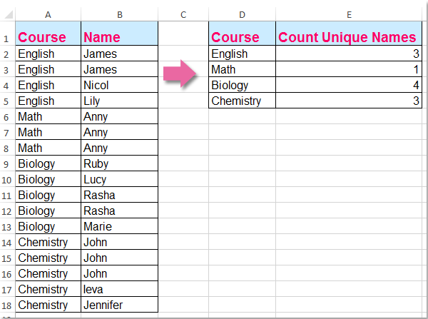
Często zdarza się, że liczymy unikalne wartości tylko w jednej kolumnie, ale w tym artykule omówię, jak liczyć unikalne wartości na podstawie innej kolumny. Na przykład mam następujące dwie kolumny danych, teraz muszę policzyć unikalne nazwy w kolumnie B na podstawie zawartości kolumny A, aby uzyskać następujący wynik:

Policz unikalne wartości na podstawie innej kolumny z formułą tablicową


strzałka niebieski prawy bąbelek Policz unikalne wartości na podstawie innej kolumny z formułą tablicową

Aby rozwiązać ten problem, pomocna może być następująca formuła, wykonaj następujące czynności:

1. Wprowadź tę formułę: =SUMPRODUCT((($A$2:$A$18=D2))/COUNTIFS($A$2:$A$18,$A$2:$A$18&"",$B$2:$B$18,$B$2:$B$18&"")) do pustej komórki, w której chcesz umieścić wynik, E2, na przykład. A następnie naciśnij Ctrl + Shift + Enter klucze razem, aby uzyskać poprawny wynik, patrz zrzut ekranu:

liczba dokumentów unikalna według kryteriów 2

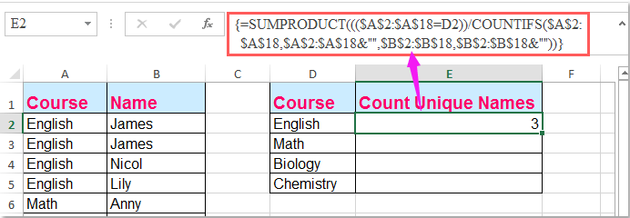
Note: W powyższym wzorze: A2: A18 to dane kolumny, na podstawie których liczysz unikalne wartości, B2: B18 to kolumna, w której chcesz policzyć unikalne wartości, D2 zawiera kryteria, na podstawie których liczysz się jako unikalne.

2. Następnie przeciągnij uchwyt wypełniania w dół, aby uzyskać unikalne wartości odpowiednich kryteriów. Zobacz zrzut ekranu:

liczba dokumentów unikalna według kryteriów 3


Podobne artykuły:

Jak policzyć liczbę unikalnych wartości w zakresie w programie Excel?

Jak liczyć unikalne wartości w przefiltrowanej kolumnie w programie Excel?

Jak policzyć te same lub zduplikowane wartości tylko raz w kolumnie?

Najlepsze narzędzia biurowe

🤖 Pomocnik AI Kutools: Zrewolucjonizuj analizę danych w oparciu o: Inteligentne wykonanie   |  Wygeneruj kod  |  Twórz niestandardowe formuły  |  Analizuj dane i generuj wykresy  |  Wywołaj funkcje Kutools...
Popularne funkcje: Znajdź, wyróżnij lub zidentyfikuj duplikaty   |  Usuń puste wiersze   |  Łącz kolumny lub komórki bez utraty danych   |   Okrągły bez wzoru ...
Super wyszukiwanie: Wiele kryteriów VLookup    Wiele wartości VLookup  |   Przeglądanie pionowe na wielu arkuszach   |   Wyszukiwanie rozmyte ....
Zaawansowana lista rozwijana: Szybko twórz listę rozwijaną   |  Zależna lista rozwijana   |  Lista rozwijana wielokrotnego wyboru ....
Menedżer kolumn: Dodaj określoną liczbę kolumn  |  Przesuń kolumny  |  Przełącz stan widoczności ukrytych kolumn  |  Porównaj zakresy i kolumny ...
Polecane funkcje: Fokus siatki   |  Widok projektu   |   Duży pasek formuły    Menedżer skoroszytów i arkuszy   |  Biblioteka zasobów (Automatyczny tekst)   |  Selektor dat   |  Połącz arkusze   |  Szyfruj/odszyfruj komórki    Wysyłaj e-maile według listy   |  Super filtr   |   Specjalny filtr (filtruj pogrubienie/kursywa/przekreślenie...) ...
15 najlepszych zestawów narzędzi12 Tekst Tools (Dodaj tekst, Usuń znaki, ...)   |   50 + Wykres rodzaje (Wykres Gantta, ...)   |   40+ Praktyczne Wzory (Oblicz wiek na podstawie urodzin, ...)   |   19 Wprowadzenie Tools (Wstaw kod QR, Wstaw obraz ze ścieżki, ...)   |   12 Konwersja Tools (Liczby na słowa, Przeliczanie walut, ...)   |   7 Połącz i podziel Tools (Zaawansowane wiersze łączenia, Podział komórki, ...)   |   ... i więcej

Zwiększ swoje umiejętności Excela dzięki Kutools for Excel i doświadcz wydajności jak nigdy dotąd. Kutools dla programu Excel oferuje ponad 300 zaawansowanych funkcji zwiększających produktywność i oszczędzających czas.  Kliknij tutaj, aby uzyskać funkcję, której najbardziej potrzebujesz...

Opis


Karta Office wprowadza interfejs z zakładkami do pakietu Office i znacznie ułatwia pracę

  • Włącz edycję i czytanie na kartach w programach Word, Excel, PowerPoint, Publisher, Access, Visio i Project.
  • Otwieraj i twórz wiele dokumentów w nowych kartach tego samego okna, a nie w nowych oknach.
  • Zwiększa produktywność o 50% i redukuje setki kliknięć myszką każdego dnia!
Comments (20)
No ratings yet. Be the first to rate!
This comment was minimized by the moderator on the site
Hi, thanks for this formula, I'm having an issue implementing it across two Worksheets. In my example, your columns A and B are on one sheet, and D and E are on another, which collects similar data from other year-based Sheets. If I put the formula on the sheet where D (Area) and E are, in E it just returns a zero =SUMPRODUCT(((MHST2324[@Team]=[@Area]))/COUNTIFS(MHST2324[@Team],MHST2324[@Team]&"",MHST2324[@School],MHST2324[@School]&"")). However if I put the formula on the Sheet where A (Team) and B (School) are, it works =SUMPRODUCT((([@Team]=Schools[Area]))/COUNTIFS([@Team],[@Team]&"",[@School],[@School]&"")), any ideas as to why?
This comment was minimized by the moderator on the site
Hey, thanks for this formula, I'm having a problem where
This comment was minimized by the moderator on the site
Классная формула, но как сделать чтобы в столбец A и B можно было постоянно добавлять и не менять формулу ? закрепить не диапазон а столбцы
This comment was minimized by the moderator on the site
Hello, DM,
In fact, you can enlarg the cell references as you need. For example:
=SUMPRODUCT((($A$2:$A$10000=D2))/COUNTIFS($A$2:$A$10000,$A$2:$A$10000&"",$B$2:$B$10000,$B$2:$B$10000&""))
Please remeber to press Ctrl + Shift + Enter keys together.
Please have a try, hope it can help you!
This comment was minimized by the moderator on the site
Is there a way to do this but not count a blank cell as a value?
This comment was minimized by the moderator on the site
Hello, MB
To count the unqiue values with criteria and skip the blank cell, you should apply the below array formula:
=SUM(--(FREQUENCY(IF($B$2:$B$15<>"",IF($A$2:$A$15=D2,MATCH($B$2:$B$15,$B$2:$B$15,0))),ROW($B$2:$B$15)-ROW(B2)+1)>0))


After pasting the fromula, please press Ctrl + Shift + Enter keys together.

https://www.extendoffice.com/images/stories/comments/comment-skyyang/doc-count-unique-criteria.png

Please try, hope it can help you!
This comment was minimized by the moderator on the site
Thank you very much for this but how does it work with a large data set. I realised it returns #N/A when the data is beyond row 78
This comment was minimized by the moderator on the site
I would need to do something similar but with dates: on a sheet in which the dates are indicated in the first column, many repeated, I would like to know how many different dates there are that meet a certain condition that appears in another column. I am applying that formula but it gives me an error. Could you help me? Thanks.
This comment was minimized by the moderator on the site
Does anyone know what the ampersand-quotes (" &"" ") in the Criteria 1 and 2 portion of the COUNTIFS formula is doing? This formula worked for me I was just hoping to understand it better.
This comment was minimized by the moderator on the site
Worked like a charm. Very much greatful to you.
This comment was minimized by the moderator on the site
OMG.... I have been searching for over a week for a formula that came close to helping me do a distinct count of one column based on another column.... YOURS FINALLY HELPED ;0) I am so happy!!!!!! Now I just need this formula that you posted to do the same thing but based on 2 column instead of one. I am going to try on my own but do you think you can help?
This comment was minimized by the moderator on the site
Hello, EB, To count the unique values based on two columns, please apply the below formula, after entering the formula, please press Ctrl + Shift + Enter keys together to get the correct result.=SUM(IFERROR(($A$2:$A$15=E2)*($B$2:$B$15=F2)/COUNTIFS($C$2:$C$15,$C$2:$C$15,$A$2:$A$15,E2,$B$2:$B$15,F2),0))
Please try, hope it can help you!
This comment was minimized by the moderator on the site
WOAH, you're a savior, thank you for sharing
This comment was minimized by the moderator on the site
Nevermind it did
There are no comments posted here yet
Load More
Please leave your comments in English
Posting as Guest
×
Rate this post:
0   Characters
Suggested Locations