Przejdź do głównej zawartości

Jak wyświetlić odpowiednią nazwę najwyższego wyniku w programie Excel?

Przypuśćmy, że mam zakres danych, który zawiera dwie kolumny - kolumnę z nazwiskiem i odpowiadającą jej kolumnę wyników, teraz chcę uzyskać nazwisko osoby, która uzyskała najwyższy wynik. Czy są jakieś dobre sposoby szybkiego rozwiązania tego problemu w programie Excel?

Wyświetl odpowiednią nazwę najwyższego wyniku za pomocą formuł


strzałka niebieski prawy bąbelek Wyświetl odpowiednią nazwę najwyższego wyniku za pomocą formuł

Aby uzyskać imię i nazwisko osoby, która uzyskała najwyższy wynik, poniższe formuły mogą pomóc w uzyskaniu wyniku.

Wprowadź tę formułę: =INDEX(A2:A14,MATCH(MAX(B2:B14),B2:B14,FALSE),)&" Scored "&MAX(B2:B14) do pustej komórki, w której chcesz wyświetlić nazwę, a następnie naciśnij Wchodzę klawisz, aby zwrócić wynik w następujący sposób:

nazwa wyświetlana doc najwyższy wynik 1

Uwagi:

1. W powyższym wzorze A2: A14 to lista nazw, z której chcesz pobrać nazwę, a B2: B14 to lista wyników.

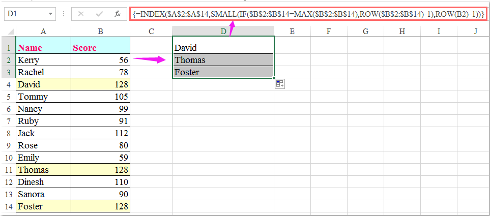
2. Powyższa formuła może uzyskać imię tylko wtedy, gdy istnieje więcej niż jedno nazwisko o takich samych najwyższych wynikach. Aby uzyskać wszystkie nazwiska, które uzyskały najwyższy wynik, skorzystaj z poniższej formuły tablicowej.

Wprowadź tę formułę:

=INDEX($A$2:$A$14,SMALL(IF($B$2:$B$14=MAX($B$2:$B$14),ROW($B$2:$B$14)-1),ROW(B2)-1)), a następnie naciśnij Ctrl + Shift + Enter klucze razem, aby wyświetlić imię, a następnie wybierz komórkę formuły i przeciągnij uchwyt wypełniania w dół, aż pojawi się wartość błędu, wszystkie nazwiska, które uzyskały najwyższy wynik, są wyświetlane jak na poniższym zrzucie ekranu:

nazwa wyświetlana doc najwyższy wynik 2

Najlepsze narzędzia biurowe

🤖 Pomocnik AI Kutools: Zrewolucjonizuj analizę danych w oparciu o: Inteligentne wykonanie   |  Wygeneruj kod  |  Twórz niestandardowe formuły  |  Analizuj dane i generuj wykresy  |  Wywołaj funkcje Kutools...
Popularne funkcje: Znajdź, wyróżnij lub zidentyfikuj duplikaty   |  Usuń puste wiersze   |  Łącz kolumny lub komórki bez utraty danych   |   Okrągły bez wzoru ...
Super wyszukiwanie: Wiele kryteriów VLookup    Wiele wartości VLookup  |   Przeglądanie pionowe na wielu arkuszach   |   Wyszukiwanie rozmyte ....
Zaawansowana lista rozwijana: Szybko twórz listę rozwijaną   |  Zależna lista rozwijana   |  Lista rozwijana wielokrotnego wyboru ....
Menedżer kolumn: Dodaj określoną liczbę kolumn  |  Przesuń kolumny  |  Przełącz stan widoczności ukrytych kolumn  |  Porównaj zakresy i kolumny ...
Polecane funkcje: Fokus siatki   |  Widok projektu   |   Duży pasek formuły    Menedżer skoroszytów i arkuszy   |  Biblioteka zasobów (Automatyczny tekst)   |  Selektor dat   |  Połącz arkusze   |  Szyfruj/odszyfruj komórki    Wysyłaj e-maile według listy   |  Super filtr   |   Specjalny filtr (filtruj pogrubienie/kursywa/przekreślenie...) ...
15 najlepszych zestawów narzędzi12 Tekst Tools (Dodaj tekst, Usuń znaki, ...)   |   50 + Wykres rodzaje (Wykres Gantta, ...)   |   40+ Praktyczne Wzory (Oblicz wiek na podstawie urodzin, ...)   |   19 Wprowadzenie Tools (Wstaw kod QR, Wstaw obraz ze ścieżki, ...)   |   12 Konwersja Tools (Liczby na słowa, Przeliczanie walut, ...)   |   7 Połącz i podziel Tools (Zaawansowane wiersze łączenia, Podział komórki, ...)   |   ... i więcej

Zwiększ swoje umiejętności Excela dzięki Kutools for Excel i doświadcz wydajności jak nigdy dotąd. Kutools dla programu Excel oferuje ponad 300 zaawansowanych funkcji zwiększających produktywność i oszczędzających czas.  Kliknij tutaj, aby uzyskać funkcję, której najbardziej potrzebujesz...

Opis


Karta Office wprowadza interfejs z zakładkami do pakietu Office i znacznie ułatwia pracę

  • Włącz edycję i czytanie na kartach w programach Word, Excel, PowerPoint, Publisher, Access, Visio i Project.
  • Otwieraj i twórz wiele dokumentów w nowych kartach tego samego okna, a nie w nowych oknach.
  • Zwiększa produktywność o 50% i redukuje setki kliknięć myszką każdego dnia!
Comments (17)
No ratings yet. Be the first to rate!
This comment was minimized by the moderator on the site
Hi sir, I tried this method, But the problem is if top two students have the same score when I look for the highest 3 one student's name alone is repeated twice with the same score instead of second student's name. How to solve this.
This comment was minimized by the moderator on the site
Hello, Divyanathan
Maybe the following array formula can help you:

=IFERROR(INDEX(A:A,SUM(IF(($B$2:$B$100+ROUND(0.1/ROW($B$2:$B$100),5))=LARGE($B$2:$B$100+ROUND(0.1/ROW($B$2:$B$100),5),ROW(A1)),ROW($B$2:$B$100)))),"")


Note: After inserting the formula, please press Ctrl + Shift + Enter keys together to get the first result, and then drga this formula cell down to get the largest n results as you need.

Please have a try, hope it can help you!
This comment was minimized by the moderator on the site
Hola disculpa me podrías apoyar para sacar la formula o otro tipo de dato que me pueda dar el nombre del tota de un resultado?

explico tengo una tabla con 4 nombres diferentes distribuidos en las celdas C3,D3,E3 y F3 de las cuales cada celda mencionada tiene rangos de productos ejemplo: detergentes
y cada celda mencionada tiene precios diferentes.
en el resultado que debo de mostrar es el valor mínimo de precio de cada detergente de las celdas ya mencionadas arriba, y a lo que quiero llegar es que indique una formula o un dato que indique que en cada resultado a la derecho me indique el nombre del valor de resultado.
muestro un ejemplo mas especifico: en la celda <C3> tiene un nombre de insumos, en la celda C4 hasta C120 están los precios de cada detergente que maneja la celda C3, en la celda <D3> esta un nombre de biodetergentes, y mismo proceso la celda D4 hasta D120 están los precios en la celda G4 se encuentra el resultado del valor mínimo de estos dos nombres (insumos-biodetergentes) teniendo el valor menor el de nombre de insumos. ahora en la celda H4 quiero que me aparezca el nombre del valor de resultado en este caso que me aparezca el nombre de "insumos" como puedo hacer para que me aparezca este nombre? espero me allá podido dar a entender de lo que requiero
muchas gracias por su atención
saludos cordiales.
This comment was minimized by the moderator on the site
ik heb het ook geprobeerd met alle dezelfde gegevens zoals in het voorbeeld maar het werkt totaal niet
This comment was minimized by the moderator on the site
Hello jac, Sorry to hear that. As I have answered in the below comment, the two formulas work great for me. And I have been wondering why the formulas aren't working for the readers. There are two reasons that can lead to the malfunction of the second formula. 
First, if you are using Excel versions before Excel 2020, then you must enter the formula =INDEX($A$2:$A$14,SMALL(IF($B$2:$B$14=MAX($B$2:$B$14),ROW($B$2:$B$14)-1),ROW(B2)-1)) via pressing Ctrl + Shift + Enter keys together.
Second, When you get the first result, remember to select the formula cell and drag the fill handle down until error value appears. So all the other results will be returned.
And as you can see in the screenshots below, the two formulas are working fine for me.  Hope my solution works. Have a nice day.
Sincerely,Mandy
This comment was minimized by the moderator on the site
bullshitdoes not work
This comment was minimized by the moderator on the site
Hello,
Sorry to hear that. But I did tried the two formulas in the article and both of them works perfectly. Please see the screenshots I uploaded here. And we would love to solve the problem for you if you can provide the details of the problem. Looking forward to your reply.Sincerely,Mandy
This comment was minimized by the moderator on the site
Trying to do the same thing but with the minimum score in Microsoft sheets. I swapped max for min as below and it didn't work =INDEX($A$2:$A$14,SMALL(IF($B$2:$B$14=MIN($B$2:$B$14),ROW($B$2:$B$14)-1),ROW(B2)-1))
This comment was minimized by the moderator on the site
Hi. This formula was exactly what I was looking for. However is there a way do this with the lowest Score but above 0 (in my case £00.00) I removed the bit of formula that displays the amount as only needed the Name and comment.I changed the MAX for MIN but there are a few entries at 0 (£00.00) and formula displays the name for the first of the '0' entries
This comment was minimized by the moderator on the site
Hello, Nigel,To lookup the lowest value above 0, you should apply the below array formula:After entering the formula, please remember to press Ctrl + Shift + Enter keys together to get the correct result.=INDEX(A2:A8,MATCH(MIN(IF(B2:B8>0,B2:B8)),B2:B8,0))&" Scored "&MIN(IF(B2:B8>0,B2:B8))
Please try, hope it can help you!
This comment was minimized by the moderator on the site
How do you find the second highest student? Please help me :( I only get the name of Thomas.
This comment was minimized by the moderator on the site
How do you find the second highest student?
This comment was minimized by the moderator on the site
How would you show two names if the high scores match?
This comment was minimized by the moderator on the site
Hello, Chris,
To get all names if there are multiple high scores match, the second formula in this article can do you a favor.
Please try it, thank you!
This comment was minimized by the moderator on the site
How would you get the matching numbers with the corresponding names to display horizontally?
There are no comments posted here yet
Load More
Please leave your comments in English
Posting as Guest
×
Rate this post:
0   Characters
Suggested Locations