Przejdź do głównej zawartości

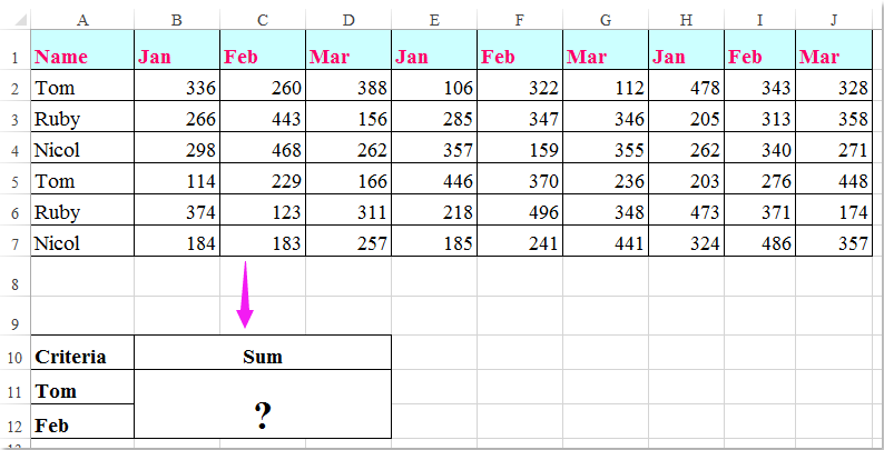
Jak sumować na podstawie kryteriów kolumn i wierszy w programie Excel? 

Mam zakres danych, który zawiera nagłówki wierszy i kolumn, teraz chcę wziąć sumę komórek, które spełniają kryteria zarówno kolumny, jak i nagłówka wiersza. Na przykład, aby zsumować komórki, których kryterium kolumny to Tom, a kryterium wiersza to luty, jak pokazano na zrzucie ekranu. W tym artykule omówię kilka przydatnych formuł, aby go rozwiązać.

kryteria sumy doc sum kolumn 1

Sumuj komórki na podstawie kryteriów kolumn i wierszy za pomocą formuł


strzałka niebieski prawy bąbelek Sumuj komórki na podstawie kryteriów kolumn i wierszy za pomocą formuł

Tutaj możesz zastosować następujące formuły, aby zsumować komórki na podstawie kryteriów kolumny i wiersza, wykonaj następujące czynności:

Wprowadź dowolną z poniższych formuł do pustej komórki, w której chcesz wyprowadzić wynik:

=SUMPRODUCT((A2:A7="Tom")*(B1:J1="Feb")*(B2:J7))

=SUM(IF(B1:J1="Feb",IF(A2:A7="Tom",B2:J7)))

A następnie naciśnij Shift + Ctrl + Enter klucze razem, aby uzyskać wynik, patrz zrzut ekranu:

kryteria sumy doc sum kolumn 2

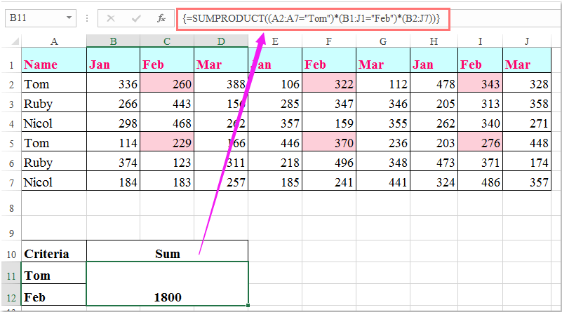
Note: W powyższych wzorach: Tomek i luty to kryteria dotyczące kolumn i wierszy oparte na A2: A7, B1: J1 czy nagłówki kolumn i nagłówki wierszy zawierają kryteria, B2: J7 to zakres danych, który chcesz zsumować.

Najlepsze narzędzia biurowe

🤖 Pomocnik AI Kutools: Zrewolucjonizuj analizę danych w oparciu o: Inteligentne wykonanie   |  Wygeneruj kod  |  Twórz niestandardowe formuły  |  Analizuj dane i generuj wykresy  |  Wywołaj funkcje Kutools...
Popularne funkcje: Znajdź, wyróżnij lub zidentyfikuj duplikaty   |  Usuń puste wiersze   |  Łącz kolumny lub komórki bez utraty danych   |   Okrągły bez wzoru ...
Super wyszukiwanie: Wiele kryteriów VLookup    Wiele wartości VLookup  |   Przeglądanie pionowe na wielu arkuszach   |   Wyszukiwanie rozmyte ....
Zaawansowana lista rozwijana: Szybko twórz listę rozwijaną   |  Zależna lista rozwijana   |  Lista rozwijana wielokrotnego wyboru ....
Menedżer kolumn: Dodaj określoną liczbę kolumn  |  Przesuń kolumny  |  Przełącz stan widoczności ukrytych kolumn  |  Porównaj zakresy i kolumny ...
Polecane funkcje: Fokus siatki   |  Widok projektu   |   Duży pasek formuły    Menedżer skoroszytów i arkuszy   |  Biblioteka zasobów (Automatyczny tekst)   |  Selektor dat   |  Połącz arkusze   |  Szyfruj/odszyfruj komórki    Wysyłaj e-maile według listy   |  Super filtr   |   Specjalny filtr (filtruj pogrubienie/kursywa/przekreślenie...) ...
15 najlepszych zestawów narzędzi12 Tekst Tools (Dodaj tekst, Usuń znaki, ...)   |   50 + Wykres rodzaje (Wykres Gantta, ...)   |   40+ Praktyczne Wzory (Oblicz wiek na podstawie urodzin, ...)   |   19 Wprowadzenie Tools (Wstaw kod QR, Wstaw obraz ze ścieżki, ...)   |   12 Konwersja Tools (Liczby na słowa, Przeliczanie walut, ...)   |   7 Połącz i podziel Tools (Zaawansowane wiersze łączenia, Podział komórki, ...)   |   ... i więcej

Zwiększ swoje umiejętności Excela dzięki Kutools for Excel i doświadcz wydajności jak nigdy dotąd. Kutools dla programu Excel oferuje ponad 300 zaawansowanych funkcji zwiększających produktywność i oszczędzających czas.  Kliknij tutaj, aby uzyskać funkcję, której najbardziej potrzebujesz...

Opis


Karta Office wprowadza interfejs z zakładkami do pakietu Office i znacznie ułatwia pracę

  • Włącz edycję i czytanie na kartach w programach Word, Excel, PowerPoint, Publisher, Access, Visio i Project.
  • Otwieraj i twórz wiele dokumentów w nowych kartach tego samego okna, a nie w nowych oknach.
  • Zwiększa produktywność o 50% i redukuje setki kliknięć myszką każdego dnia!
Comments (17)
No ratings yet. Be the first to rate!
This comment was minimized by the moderator on the site
Brilliant!

The function =SUM(IF(B1:J1="Feb",IF(A2:A7="Tom",B2:J7))) is a great X & Y summation tool.
I would not have thought this logic out on my own.
In fact i took me a minute to deconstruction the operations.

Thank you
This comment was minimized by the moderator on the site
My data that I am trying to retrieve is in a table. Would this impact the result at all? I have:

=SUM(IF('[Primary Controller Active Project Database (KC notes)1.xlsx]Active Project Tracking'!$B2:$B66=X2,IF('[Primary Controller Active Project Database (KC notes)1.xlsx]Active Project Tracking'!$A1:$AV1=AH10,'[Primary Controller Active Project Database (KC notes)1.xlsx]Active Project Tracking'!$H$2:$AV$66)))

So I think the equivalent would be if you did your information above, but in a table in a different workbook. Thoughts?
This comment was minimized by the moderator on the site
If there were negatives in the matrix and you only wanted to include the positives, what would you do? 
I tried to do something like this:

=SUMPRODUCT((Column = Criteria)* ( Row = Criteria) * (second column = Criteria) * (Matrix) * (Matrix >0))

This comment was minimized by the moderator on the site
Is there a way to do this but instead of writing "Tom" & "Feb" in the formula, you are able to reference the criteria cells e.g.A11 & A12?
This comment was minimized by the moderator on the site
Hello, Rianna,Yest, as you said, you can use the cell references to replace the text in the formula, such as:
=SUMPRODUCT((A2:A7=A2)*(B1:J1=C1)*(B2:J7))
=SUM(IF(B1:J1=C1,IF(A2:A7=A2,B2:J7)))
This comment was minimized by the moderator on the site
In the above example which formula should I use if I wanted calculate the sum of the amounts earned by Tom Ruby & Nicol in March?
This comment was minimized by the moderator on the site
Hello, Nabar,To get the result you want, please apply the below formula:=SUMPRODUCT(((A2:A7="Tom")+(A2:A7="Nicol")+(A2:A7="Ruby"))*(B1:J1="Mar")*(B2:J7))
Please try, hope it can help you!
This comment was minimized by the moderator on the site
Hello Skyyang,
Thank you for your response. I tried the formula you suggested but I am not getting the right answer. Probably I wasn't able to put my query correctly. Let me try again I have a spreadsheet with data with daily calculation, I have numbered the first row 1,2,3,4.....132. 2nd, 3rd 4th &5th rows has table headings. The first column has line no's numbered 1, 2,3,.....3005 starting from row 6,range B6:EF3005 has data filled in on everyday basis. In second sheet i have a table in which I want to apply a formula which will look up two line numbers fed in two different rows and calculate the sum from the range B6: EF3005 from the data spreadsheet between the two line numbers from a certain column viz sum of values in column 15 between rows (line No's) 50 & 85.
This comment was minimized by the moderator on the site
Is there a way to make this work with wildcard characters? I'd like to use it on everything starting with certain characters, but with (a fixed number of) undefined characters at the end, i.e. =SUM(IF(B1:J1="Fe*",IF(A2:A7="To*",B2:J7)))
This comment was minimized by the moderator on the site
Should anyone have the same question, this is how I solved it (in Google Sheets, not tested in Excel):

=ArrayFormula(SUM(IF(regexmatch(O5:W5,"^Fe."),IF(regexmatch(N6:N11,"^To."),O6:W11))))

Note that the IF function does not support wildcard characters and that for regexmatch the wildcards are different and can be found here: https://github.com/google/re2/blob/master/doc/syntax.txt
In this particular instance, I used ^ to indicate that Fe & Tom occur at the beginning of text and . to allow for any following character (* would mean zero or more of the previous character, e.g. Fe* would only look for instances with 1 or more "e"s after F)
This comment was minimized by the moderator on the site
I tried to create a formula to calculate if the D12 is blank, it will calculate from K12 to AH12 but it seems this part ' regexmatch(D12,"")' is not working
ArrayFormula(SUM(IF(regexmatch(D12,""),K12:AH12)))
This comment was minimized by the moderator on the site
Thank you so much! You made my day!! @TeSageDS
This comment was minimized by the moderator on the site
how would you do this same formula if you wanted to sum both Feb and March together? please help! thanks

=SUMPRODUCT((A2:A7="Tom")*(B1:J1="Feb")*(B2:J7))
This comment was minimized by the moderator on the site
Hello,Angela,
To solve your problem, you just need to apply the below formula, please try it.

=SUMPRODUCT((A2:A7="Tom")*((B1:J1="Feb")+(B1:J1="Mar"))*(B2:J7)).

Hope it can help you!
This comment was minimized by the moderator on the site
Brilliant
This comment was minimized by the moderator on the site
Worth pointing out that of the two formulas provided above you do not need to enter the SUMPRODUCT formula with Ctrl + Shift + Enter. It will work perfectly well without it.
This comment was minimized by the moderator on the site
Awesome, this is the one what i was looking for. thanks for the help
There are no comments posted here yet
Please leave your comments in English
Posting as Guest
×
Rate this post:
0   Characters
Suggested Locations