Przejdź do głównej zawartości

Jak pominąć zwracanie wielu kolumn z tabeli programu Excel?

W arkuszu programu Excel można zastosować funkcję Vlookup, aby zwrócić pasującą wartość z jednej kolumny. Ale czasami może być konieczne wyodrębnienie dopasowanych wartości z wielu kolumn, jak pokazano na zrzucie ekranu. W jaki sposób można uzyskać odpowiednie wartości w tym samym czasie z wielu kolumn za pomocą funkcji Vlookup?

doc vlookup wiele kolumn 1

Vlookup, aby zwrócić pasujące wartości z wielu kolumn z formułą tablicową


Vlookup, aby zwrócić pasujące wartości z wielu kolumn z formułą tablicową

Tutaj przedstawię funkcję Vlookup, która zwraca dopasowane wartości z wielu kolumn, wykonaj następujące czynności:

1. Wybierz komórki, w których chcesz umieścić pasujące wartości z wielu kolumn, zobacz zrzut ekranu:

doc vlookup wiele kolumn 2

2. Następnie wprowadź tę formułę: =VLOOKUP(G2,A1:E13,{2,4,5},FALSE) do paska formuły, a następnie naciśnij Ctrl + Shift + Enter klucze razem, a pasujące wartości z wielu kolumn zostały wyodrębnione jednocześnie, patrz zrzut ekranu:

doc vlookup wiele kolumn 3

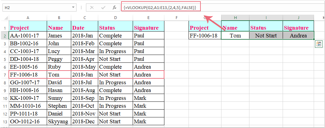
Note: W powyższym wzorze, G2 to kryteria, na podstawie których chcesz zwracać wartości, A1: E13 to zakres tabeli, z którego chcesz przeglądać, liczba 2, 4, 5 to numery kolumn, z których chcesz zwrócić wartości.

Najlepsze narzędzia biurowe

🤖 Pomocnik AI Kutools: Zrewolucjonizuj analizę danych w oparciu o: Inteligentne wykonanie   |  Wygeneruj kod  |  Twórz niestandardowe formuły  |  Analizuj dane i generuj wykresy  |  Wywołaj funkcje Kutools...
Popularne funkcje: Znajdź, wyróżnij lub zidentyfikuj duplikaty   |  Usuń puste wiersze   |  Łącz kolumny lub komórki bez utraty danych   |   Okrągły bez wzoru ...
Super wyszukiwanie: Wiele kryteriów VLookup    Wiele wartości VLookup  |   Przeglądanie pionowe na wielu arkuszach   |   Wyszukiwanie rozmyte ....
Zaawansowana lista rozwijana: Szybko twórz listę rozwijaną   |  Zależna lista rozwijana   |  Lista rozwijana wielokrotnego wyboru ....
Menedżer kolumn: Dodaj określoną liczbę kolumn  |  Przesuń kolumny  |  Przełącz stan widoczności ukrytych kolumn  |  Porównaj zakresy i kolumny ...
Polecane funkcje: Fokus siatki   |  Widok projektu   |   Duży pasek formuły    Menedżer skoroszytów i arkuszy   |  Biblioteka zasobów (Automatyczny tekst)   |  Selektor dat   |  Połącz arkusze   |  Szyfruj/odszyfruj komórki    Wysyłaj e-maile według listy   |  Super filtr   |   Specjalny filtr (filtruj pogrubienie/kursywa/przekreślenie...) ...
15 najlepszych zestawów narzędzi12 Tekst Tools (Dodaj tekst, Usuń znaki, ...)   |   50 + Wykres rodzaje (Wykres Gantta, ...)   |   40+ Praktyczne Wzory (Oblicz wiek na podstawie urodzin, ...)   |   19 Wprowadzenie Tools (Wstaw kod QR, Wstaw obraz ze ścieżki, ...)   |   12 Konwersja Tools (Liczby na słowa, Przeliczanie walut, ...)   |   7 Połącz i podziel Tools (Zaawansowane wiersze łączenia, Podział komórki, ...)   |   ... i więcej

Zwiększ swoje umiejętności Excela dzięki Kutools for Excel i doświadcz wydajności jak nigdy dotąd. Kutools dla programu Excel oferuje ponad 300 zaawansowanych funkcji zwiększających produktywność i oszczędzających czas.  Kliknij tutaj, aby uzyskać funkcję, której najbardziej potrzebujesz...

Opis


Karta Office wprowadza interfejs z zakładkami do pakietu Office i znacznie ułatwia pracę

  • Włącz edycję i czytanie na kartach w programach Word, Excel, PowerPoint, Publisher, Access, Visio i Project.
  • Otwieraj i twórz wiele dokumentów w nowych kartach tego samego okna, a nie w nowych oknach.
  • Zwiększa produktywność o 50% i redukuje setki kliknięć myszką każdego dnia!
Comments (15)
No ratings yet. Be the first to rate!
This comment was minimized by the moderator on the site
how can i search for multiple lookup value?for eg: these two arrays shows diff freq coumn,gain,veritcal BW,tolerance etc.I want to get an average values gain and 3db BW..how can i enter the formula
y1    1800    7.5dBi +/- 2.9    22.1° +/- 6.8        7.5
y1    1900    7.6dBi +/- 3.0    18.9° +/- 3.6        7.6
y1    2100    6.7dBi +/- 2.6    17.7° +/- 3.6        6.7
y1    AWS    7.2dBi +/- 2.8    20.4° +/- 9.4        7.2
y1    2300    8.3dBi +/- 3.6    15.8° +/- 1.6        8.3
y1    2600    7.9dBi +/- 2.4    17.1° +/- 1.7        7.9
y2    1800    6.9dBi +/- 1.4    27.1° +/- 10.8        6.9
y2    1900    6.9dBi +/- 1.5    23.0° +/- 12.5        6.9
y2    2100    7.6dBi +/- 2.3    21.7° +/- 19.6        7.6
y2    AWS    8.0dBi +/- 2.5    23.3° +/- 13.8        8
y2    2300    7.7dBi +/- 1.6    15.9° +/- 5.9        7.7
y2    2600    6.5dBi +/- 2.3    14.5° +/- 3.9        6.5
This comment was minimized by the moderator on the site
I have many rows with same value but need to get multiple value after look up, I need to get two different EO ref , how can U##TRX EO
HXPRE-MQ1371 AB0024822
This comment was minimized by the moderator on the site
Thank you!! The { } of the columns is what I was missing. Appreciate this page!
This comment was minimized by the moderator on the site
Thanks! Super helpful, when other online options weren't
This comment was minimized by the moderator on the site
What if you need to have multiple rows as well? Ex. find all the FF-1006-18 rows while still only bringing back column B, D, and E.
This comment was minimized by the moderator on the site
Hello, Shelly,
Maybe there is not a direct formula for helping you, but, you can apply the below array fromula to get all matching values from the entire row, and then delete or hide the unwanted column as you need.
=INDEX($A$2:$E$10, SMALL(IF($G$2=$A$2:$A$10, ROW($A$2:$A$10)-MIN(ROW($A$2:$A$10))+1, ""), ROW(B1)),COLUMN(B1))
Then press Ctrl + Shift + Enter keys to get the first cell and then drag the fill handle to right and then drga down to get all corresponding values.

Please try, hope it can help you!
This comment was minimized by the moderator on the site
Thanks! This was really Helpful!
This comment was minimized by the moderator on the site
This method does not work. Even if it did, it is not the proper method.
Example of correct method is:
VLOOKUP($A2:$A1093, '[Workbook1.xlsx]Sheet2'!$A$2:$D$111,COLUMN(G2),FALSE)

Make sure you add $ before the column letter of your lookup reference to make sure it remains static, once done, using the filler button on the selected target cell, drag right to the corresponding number of columns.
This comment was minimized by the moderator on the site
This comment is exactly what I needed
This comment was minimized by the moderator on the site
How can I do this using 2 different spread sheets?
This comment was minimized by the moderator on the site
Hello, Lana,
The above formula in this article also can help you to get the results in another worksheet, you just need to change the cell reference as follows:
=VLOOKUP(A1,Sheet1!A1:E13,{2,4,5},FALSE)
Please remember to press Ctrl + Shift + Enter keys together to get the correct results.
This comment was minimized by the moderator on the site
NOT GETTING MULTIPLE COLUMN I'M GETTING ONLY ONE COLUMN VALUE
This comment was minimized by the moderator on the site
Hi, HARI,
To apply this formula, first, you should select the multiple cells where you want to output the results, and then copy the formula into the formula bar, then press Ctrl + Shift + Enter keys together to get the results.
Please try, hope it can help you!
This comment was minimized by the moderator on the site
This is great. How do I carry this formula down if I have 10,000 rows? I've tried a few ways but of course it's changing the formula on me.
This comment was minimized by the moderator on the site
Hi, Scully,
To apply this formula to multiple rows, you just need to change the relative cell reference to absolute reference, as this: =VLOOKUP(A1,Sheet1!$A$1:$E$13,{2,4,5},FALSE).
Please try this, hope it can help you!
There are no comments posted here yet
Please leave your comments in English
Posting as Guest
×
Rate this post:
0   Characters
Suggested Locations